What I want to do is to simulate exactly the shaking of the spring in this animation:

The way I thought to do this is to split the gif into frames (30 frames in total). Then I took the spring position in each frame and calculated the difference of the spring position in each frame from the previous position (for example springPosition1 - springPosition0). The graph of all these differences looks like this:

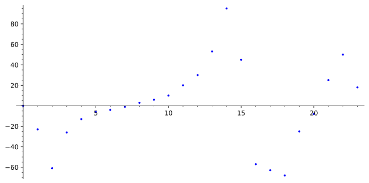
I constructed this graph as an approximately cubic bezier curve. Then, since the first derivative of each point of the curve represents the velocity, I thought to add the first derivative of each point to the position of the spring:

var total_delta: float = 0
func _physics_process(delta):
   spring.position.y += Bezier.get_velocity(total_delta)
   total_delta += delta

Here is the animation I got:

As you can see, I did not achieve the desired result. Where do you think the problem lies? My guess is that the curve I showed above needs more zigzags to be like a spring. It seems strange to me that there are so few zigzags, but this is what a position-time graph looks like. It confuses me that the animation is not accurate but the position-time graph is. What solution would you suggest to make this animation?

Darksiders said:
What solution would you suggest to make this animation?

I would just simulate the spring physics instead trying to reverse engineer it. The former seems too simple to make the latter trouble worth it. Simulating the middle point of the rope would be enough for the shown image.

It should be also possible to turn spring physics into a simple function. I have seen this often iirc, but actually i don't know spring damper math, and pulling something out of my nose i would get something like this:

https://graphtoy.com/?f1(x,t)=cos(x*x)%20/%20(1+x*x)&v1=true&f2(x,t)=&v2=false&f3(x,t)=&v3=false&f4(x,t)=&v4=false&f5(x,t)=&v5=false&f6(x,t)=&v6=false&grid=1&coords=5.497814800458062,-3.0745282187371967,7.451055876709862​

It shows oscillations of decreasing amplitude and increasing frequency over time. But there surely is a proper formula showing procedurally generated and realisitc spring physics. Animation guys should know.

Darksiders said:
I constructed this graph as an approximately cubic bezier curve. Then, since the first derivative of each point of the curve represents the velocity, I thought to add the first derivative of each point to the position of the spring:

Cubic bezier is not really an easy tool to smooth out sample data. Catmull-Rom does that ‘automatically’ without raising questions on knots vs. tangent handles and continuity.
Bit even then you would need a higher resolution of samples where the signal isn't smooth. It looks like your measuered plot of samples already undersamples the true signal, maybe because the gif is low fps.
But as said, doing just ‘the right thing’ surely is easier.

Just found some code example here: https://blog.maximeheckel.com/posts/the-physics-behind-spring-animations/​

They confuse ‘framerate’ with timestep or deltatime, but nice otherwise.