The use case is that, as usual, I'm writing a client for Second Life/Open Simulator, which has both legacy bump maps and newer normal maps. The old SL renderer uses a different shader for bump maps for historical reasons. I want to convert them into texture maps once, when loaded, and use the same render pipeline as for everything else.
JoeJ said: You get higher quality from a larger kernel at the cost of loosing high frequencies, proven from the rounding of the tiles at the bottom image. Notice this rounding does not agree with the grid image on the right, which is just black and white.
Which is why I said you can do a weighted combination of derivatives at different scales to get the desired look for each texture. You can choose to weight the 1-pixel scale derivative higher than others to emphasize the small details, or use the bigger derivatives to emphasize the 3D shape of the bump map. In my implementation I control this with a “balance” parameter that adjusts the weight between fine details and big features, using several different derivative octaves (e.g. 1px, 2px, 4px, 8px, 16px, 32px, etc.). The images I posed above were generated with equal balance of low and high frequencies.
@aressera I agree your proposal is better in practice for normal maps, as it allows to tweak for the best compromise. But for other applications going with simple and fast gradients is the better option, and i got a bit ignorant while focusing on the problem to do this as good as possible. Sorry for that. ; )
I did the test code, and found two surprises, lacking an explanation for either of them. Here's what gave me best results:
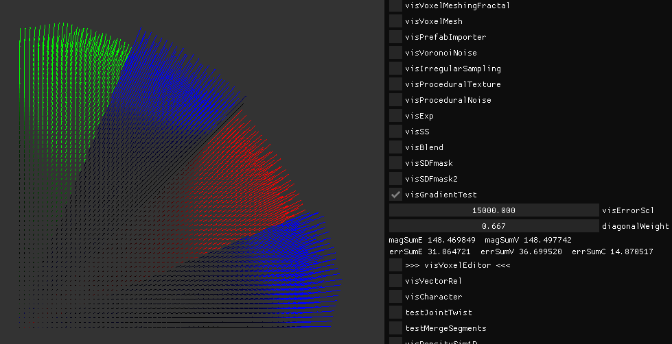
The red color shows error of direct neighbors only (E), green is error for diagonals (V), and blue is best case for combining both (C). Accumulated angle error numbers printed on the right. So we see using both reduces the error to one half, and errors are noticeable mostly on the edge of the sphere at steep angles.
The confusing finds:
I got clearly best results with a weight of ⅔ for the diagonals, not ½ as i had assumed.
To make magnitudes of diagonal gradients similar to direct neighbor gradients, i had to multiply with 0.5, not 1/sqrt(2)
That's interesting. Now i'll have to do the same test in 3D too, but then i can probably improve the quality of my fluid simulations by using different weights… : )
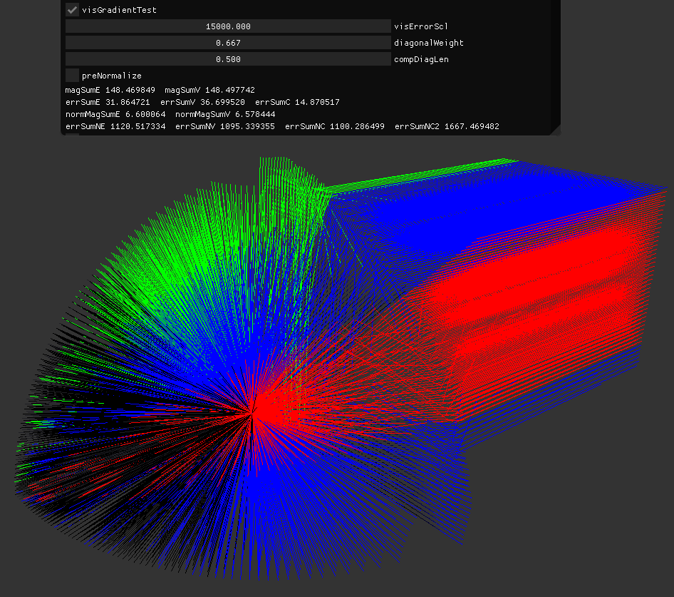
I have now added normals calculation, giving no further surprises.
Error is smaller by summing up weighted cross products than from summing normalized cross products. For squared error it's the opposite, but the difference is tiny, and it looks like erroneous normals at the discontinuous boundary are the cause.
So that's the most accurate normals from a height map i can get without any filtering. (Removing code from previous post.)
Edit: Changed the code to do error measurement only if the sample is on the sphere, otherwise the reference normal is wrong and we got big error numbers. Now the squared error also agrees with not pre-normalizing.