
Spatial interpolation of scattered data is a vital technique used in graphics programming, games, medical, scientific applications, mining, weather forecasting etc. Some of the most widely used techniques are:
- Inverse distance weighting
- Natural neighbour interpolation
- Kriging
Here I will discuss a cunning optimization of discrete natural neighbour interpolation, introduced by Sibson (1981).
Natural neighbour interpolation produces a pleasing result and by its nature deals with a few potential 'gotchas' in spatial interpolation. However in reference form it is very slow, hence the interest in finding faster methods / variations.
Natural neighbour interpolation is a simple extension to the idea of Voronoi tessellation (aka Dirichlet tessellation). A Voronoi tessellation can be constructed by simply assigning each cell on a grid to the nearest data point. It can also be calculated geometrically.
As it is, Voronoi tessellation provides for missing values between data points, but the boundaries between tiles are sharp. In order to blend between them, Sibson suggested inserting each pixel to be tested as a new data point, constructing the new Voronoi tessellation, and mapping out which areas are 'stolen' from neighbours. The influence of each neighbour is then weighted by the size of the area stolen.
This can be done geometrically, or by discrete methods (i.e. using a grid). The discrete method becomes more efficient with large numbers of data points, however it can be very slow with sparse data points. It should also be born in mind that it is an approximation (the accuracy depending on the size of the tesselated areas : hence the density of points and the size of the grid).
The obvious algorithm would be something like as follows:
- Construct Voronoi tessellation of data points on a grid, marking which data point 'owns' each cell.
- For each cell to be interpolated, flood outward and add the influence of each cell 'stolen' from a neighbouring data point.
- Once all cells that are closer to the test cell are found, divide the total influence by the number of stolen cells to get the interpolated value.
This works, but is very slow.
Park et al (2006) introduced a new way of calculating the solution, using the brute force processing power of GPUs. Essentially they realised that instead of calculating the 'gather' for each cell, the problem could be turned on its head, instead calculating the 'scatter' from each cell, which will always be a circle (or sphere, as this works in 3d and higher dimensions) with a radius equal to the distance to the closest neighbour. This is best explained by reference to the Park et al paper rather than giving a full explanation here.
These simple circles of scatter can more easily be calculated than the irregular Voronoi tiles and can be accelerated by rendering the scatter onto a grid using the GPU, and accumulating the influence at each cell.
For my libraries I was interested in ways of speeding up the process, without using the GPU.
Bulk Spheres
I tried several approaches (gather and scatter). In the end my favourite was a simple modification of Park et al's scatter technique. While the GPU works well at rendering circular areas, I wanted to minimize the monkey work the CPU was doing when following the same approach. I realised that when rendering the scatter 'spheres' from neighbouring cells, by far the majority of the sphere would have been already covered by the previous scatter. Was there some way of combining these 'renders' so I did more work at the same time?
As it was, there was a way I came up with to combine them. First I grouped cells into a coarser grid that lay across the first. The number of cells to consolidate into one new cell could be varied in the code, I would use say (in 2d) 9 cells, 16 cells, 25 cells etc.
Then as a preprocess for each coarse grid cell, I would precalculate the radius of a 'bulk sphere' (centred in the centre of the coarse grid cell) that would encompass some of the area used by each scatter sphere (from the cells making up the coarse cell). The bulk sphere would always be smaller than the actual scatter sphere, but provided all the cells in the coarse cell had the same owner (data point), I could calculate all their effects in one pass - essentially doing 9 / 16 / 25 times the work in one pass!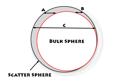
However, there is one complication, we must now deal with the small areas of the scatter sphere that are not drawn by the bulk sphere. But this is possible. The process is thus:
1) Create a coarse grid from the main grid
2) Calculate bulk spheres from the scatter spheres
3) Apply the bulk spheres to the accumulating grid result
4) Apply the 'leftovers' for each of the main grid cells
How to calculate the leftovers becomes simpler when we look at a simple optimization for rendering each y line of the spheres:
Instead of naively calculating the distance to the sphere centre for each cell when rendering (to decide whether a cell is part of the sphere or not), we can calculate the starting x coord and ending x coord for each y line. This can be done using some handy maths:
x_offset_sqr = radius_sqr - (y * y)
Then a whole line can be rendered in one go, without any testing per cell.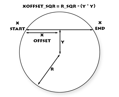
This same technique can be used to find the xstart and xend of the bulk sphere as well! So instead of rendering the whole line the process becomes:
- Render line start segment (xstart -> bulk sphere x start)
- Render line end segment (bulk sphere x end -> xend)
Using this technique the results are identical to the reference implementation, but can be significantly faster, 2 to several times faster depending on the input data. This could potentially be useful in many scenarios as it is essentially a 'free' speedup. I have not investigated whether it could be used to speed up the GPU implementation.
Finally I would like to introduce a modification to natural neighbour scheme.
Voronoi tessellations and natural neighbourhoods are used in part because they are conceptionally simple. They may also give a good approximation of natural processes where substances move at approximately fixed speed, such as diffusion during organism development. However, because of their apparent simplicity, there is a danger of overbiasing towards their use when other methods may be more appropriate. The main problem with natural neighbour interpolation is that it is slow to calculate. Instead of finding faster ways to calculate it, we should also be putting effort to finding other sensible more computationally efficent ways of interpolating data.
Here I would like to suggest a simple modification which produces approximately similar results, but runs orders of magnitude faster.
First, an observation. The speed of discrete natural neighbour interpolation is directly related to the density of the data points. Rendering either scatter or gather, the amount of time needed for each cell raises as the square of the distance between points (or the cube in 3d). This leads to pathologically long runtimes in sparse areas of the grid.
Incremental Natural Neighbour Interpolation
Instead, I suggest a better interpolator should be able to incrementally add calculated interpolated points TO THE INPUT DATA, and use calculated points to further calculate the later points. If instead of calculating points in order across the grid, we first calculate points IN FREE SPACE, we will significantly increase the overall density as we go, and thus the speed of calculation will INCREASE as the grid is calculated.
When I tried this method I found two things. Firstly, it works. It runs like sh*t off a shovel. Secondly, it reveals a 'flaw' in natural neighbourhood interpolation. When you add 'in between' calculated points, the final result is NOT the same as the reference implementation. The best solution, to my mind, is to come up with a measure that produces the same result when using 'inbetweeners' as using a reference implementation. I will leave this as an exercise for readers.
Having said that, it is possible to get reasonable results using this incremental method, certainly suitable for realtime application and rapid visualization where absolute accuracy is not paramount.
My first implementation of the incremental method I first calculated points at random across the grid. This works but gives slightly differing results each time, depending on the random seed. Looking for a more consistent method I next tried a regular grid pattern. This works too but the end result has the 'look' of a grid.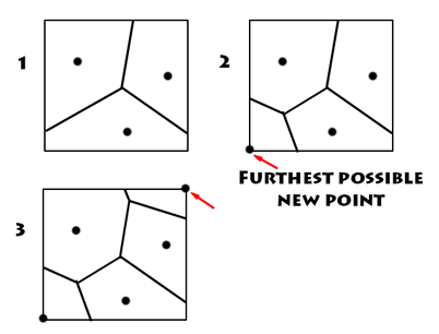
My final implementation was something that to me makes 'sense' spatially. Each cell I interpolated in turn (and added to the input points) I chose by choosing the cell that was FURTHEST from all the data points. This is also (coincidentally) the point that will give the greatest speedup to later added points. This means after the first few added points there is a massive speedup occurring. The only downside is some extra data is needed for housekeeping for making sure I am choosing the furthest cell each time.
The results also look visually pleasing, although the best number of these points to add may vary according to the grid size / data.
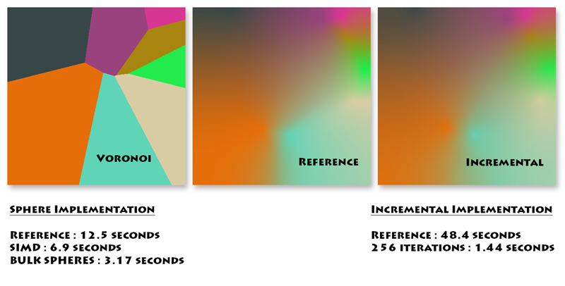
The diagram shows some of my results. The absolute times are not vitally important, but the relative differences between the methods are indicative. The incremental technique is easily the fastest, and has not been heavily optimized.
I would add that I am not a mathematician nor an expert in this field, but hopefully some of these ideas will be of interest to those working in it and spur further work.
References
1. Sibson, R. (1981). "A brief description of natural neighbor interpolation (Chapter 2)". In V. Barnett. Interpreting Multivariate Data. Chichester: John Wiley. pp. 21-36.
2. Park, S. W., Linsen, L., Kreylos, O., Owens, J. D., and Hamann B. (2006). "Discrete sibson interpolation". IEEE Transactions on Visualization and Computer Graphics 12, 2 (Mar./ Apr.), 243-253.
