physicist and member of
No Bucks Racing Club

P.O. Box 662
Burbank, CA 91503

(C)Copyright 1991

We found in part 5 of this series, "Introduction to the Racing Line," that a driver can lose a shocking amount of time by taking a bad line in a corner. With a six-foot-wide car on a ten-foot-wide course, one can lose sixteen hundredths by 'blowing' a single right-angle turn. This month, we extend the analysis of the racing line by following our example car down a straight. It is often said that the most critical corner in a course is the one before the longest straight. Let's find out how critical it is. We calculate how much time it takes to go down a straight as a function of the speed entering the straight. The results, which are given at the end, are not terribly dramatic, but we make several, key improvements in the mathematical model that is under continuing development in this series of articles. These improvements will be used as we proceed designing the computer program begun in Part 8.

The mathematical model for traveling down a straight follows from Newton's second law:



where is the force on the car, is the mass of the car, and is the acceleration of the car. We want to solve this equation to get time as a function of distance down the straight. Basically, we want a table of numbers so that we can look up the time it takes to go any distance. We can build this table using accountants' columnar paper, or we can use the modern version of the columnar pad: the electronic spreadsheet program.

To solve equation 1 , we first invert it:



Now , the acceleration, is the rate of change of velocity with time. Rate of change is simply the ratio of a small change in velocity to a small change in time. Let us assume that we have filled in a column of times on our table. The times start with and go up by the same, small amount, say sec. Physicists call this small time the integration step. It is standard practice to begin solving an equation with a fixed integration step. There are sometimes good reasons to vary the integration step, but those reasons do not arise in this problem. Let us call the integration step . If we call the time in the -th row , then for every row except the first,



We label another column velocity, and we'll call the velocity in the -th row . For every row except the first, equation 2 becomes:



We want to fill in velocities as we go down the columns, so we need to solve equation 4 for . This will give us a formula for computing given for every row except the first. In the first row, we put the speed with which we enter the straight, which is an input to the problem. We get:



We label another column distance, and we call the distance value in the -th row . Just as acceleration is the rate of change of velocity, so velocity is the rate of change of distance over time. Just as before, then, we may write:



Solved for , this is:



Equation 7 gives us a formula for calculating the distance for any time given the previous distance and the velocity calculated by equation 5 . Physicists would say that we have a scheme for integrating the equations of motion.

A small detail is missing: what is the force, ? Everything to this point is kinematic. The real modeling starts now with formulas for calculating the force. For this, we will draw on all the previous articles in this series. Let's label another column force, and a few more with drag, rolling resistance, engine torque, engine rpm, wheel rpm, trans gear ratio, drive ratio, wheel torque, and drive force. As you can see, we are going to derive a fairly complete, if not accurate, model of accelerating down the straight. We need a few constants:



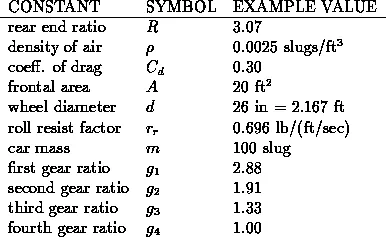
and a few variables:



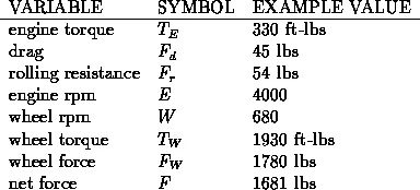
All the example values are for a late model Corvette. Slugs are the English unit of mass, and 1 slug weighs about 32.1 lbs at sea level (another manifestation of , with in lbs, in slugs, and being the acceleration of gravity, 32.1 ft/sec).

The most basic modeling equation is that the force we can use for forward acceleration is the propelling force transmitted through the wheels minus drag and rolling resistance:



The force of drag we get from Part 6:



Note that to calculate the force at step , we can use the velocity at step . This force goes into calculating the acceleration at step , which is used to calculate the velocity and distance at step by equations 5 and 7 . Those two equations represent the only 'backward references' we need. Thus, the only inputs to the integration are the initial distance, 0, and the entrance velocity, .

The rolling resistance is approximately proportional to the velocity:



This approximation is probably the weakest one in the model. I derived it by noting from a Corvette book that 8.2 hp were needed to overcome rolling resistance at 55 mph. I have nothing else but intuition to go on for this equation, so take it with a grain of salt.

Finally, we must calculate the forward force delivered by the ground to the car by reaction to the rearward force delivered to the ground via the engine and drive train:



This equation simply states that we take the engine torque multiplied by the rear axle ratio and the transmission drive ratio in the -th gear, which is the torque at the drive wheels, , and divide it by the radius of the wheel, which is half the diameter of the wheel, .

To calculate the forward force, we must decide what gear to be in. The logic we use to do this is the following: from the velocity, we can calculate the wheel rpm:



From this, we know the engine rpm:



At each step of integration, we look at the current engine rpm and ask "is it past the torque peak of the engine?" If so, we shift to the next highest gear, if possible. Somewhat arbitrarily, we assume that the torque peak is at 4200 rpm. To keep things simple, we also make the optimistic assumption that the engine puts out a constant torque of 330 ft-lbs. To make the model more realistic, we need merely look up a torque curve for our engine, usually expressed as a function of rpm, and read the torque off the curve at each step of the integration. The current approximation is not terrible however; it merely gives us artificially good times and speeds. Another important improvement on the logic would be to check whether the wheels are spinning, i.e., that acceleration is less than about , and to 'lift off the gas' in that case.

We have all the ingredients necessary to calculate how much time it takes to cover a straight given an initial speed. You can imagine doing the calculations outlined above by hand on columnar paper, or you can check my results (below) by programming them up in a spreadsheet program like Lotus 1-2-3 or Microsoft Excel. Eventually, of course, if you follow this series, you will see these equations again as we write our Scheme program for simulating car dynamics. Integrating the equations of motion by hand will take you many hours. Using a spreadsheet will take several hours, too, but many less than integrating by hand.

To illustrate the process, we show below the times and exit speeds for a 200 foot straight, which is a fairly long one in autocrossing, and a 500 foot straight, which you should only see on race tracks. We show times and speeds for a variety of speeds entering the straight from 25 to 50 mph in Table 1 . The results are also summarized in the two plots, Figures 1 and 2 .







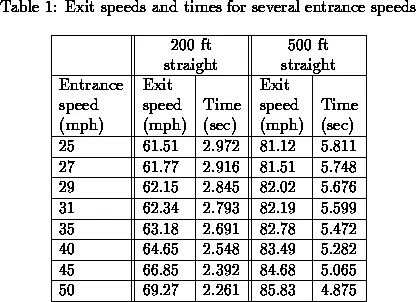
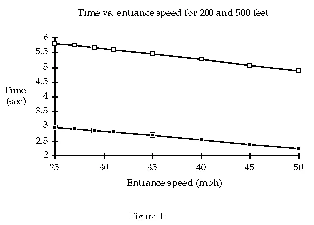
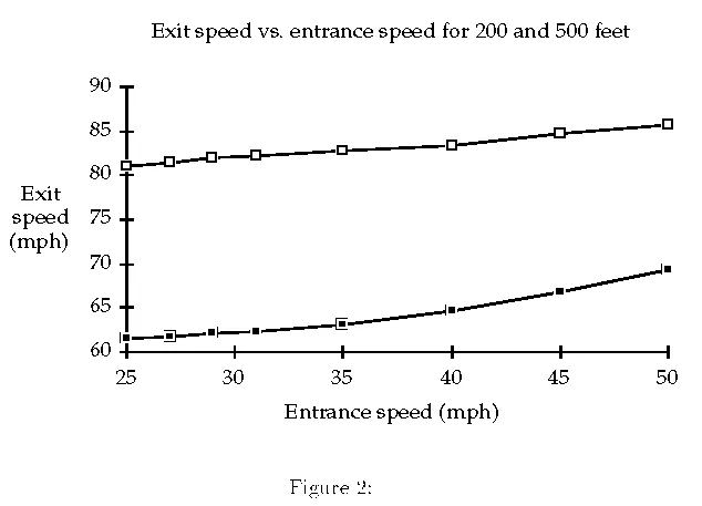
The notable facts arising in this analysis are the following. The time difference resulting from entering the 200' straight at 27 mph rather than 25 mph is about 6 hundredths. Frankly, not as much as I expected. The time difference between entering at 31 mph over 25 mph is about 2 tenths, again less than I would have guessed. The speed difference at the end of the straight between entering at 25 mph and 50 mph is only 8 mph, a result of the fact that the car labors against friction and higher gear ratios at high speeds. It is also a consequence of the fact that there is so much torque available at 25 mph in low gear that the car can almost make up the difference over the relatively short 200' straight. In fact, on the longer 500' straight, the exit speed difference between entering at 25 mph and 50 mph is not even 5 mph, though the time difference is nearly a full second.

This analysis would most likely be much more dramatic for a car with less torque than a Corvette. In a Corvette, with 330 ft-lbs of torque on tap, the penalty for entering a straight slower than necessary is not so great as it would be in a more typical car, where recovering speed lost through timidity or bad cornering is much more difficult.

Again, the analysis can be improved by using a real torque curve and by checking whether the wheels are spinning in lower gears.

[hr]
converted by: rck@home.net
Thu Sep 29 14:11:00 PDT 1994