Physics simulations commonly use the Coulomb friction model, which requires a coefficent of friction between the materials of two interacting objects to calculate the friction force. Similarly, a coefficient of restitution is required to calculate the collision response force. But how do you determine these coefficients for each pair of materials?
A common approach is to define values of friction and restitution for each individual material and then combine them to get the material-material values. Given individual material friction values \(x\) and \(y\), we need to define a combination function \(f(x,y)\). Similarly, \(r(x,y)\) for restitution (using \(x\) and \(y\) to mean the material restitution values this time).
Function requirements
The value of \(f(x,y)\) and \(r(x,y)\) should lie between \(x\) and \(y\). So \(f(x,x) = x\) and \(r(x,x) = x\).
For any constant \(c\), \(f(x,c)\) and \(r(x,c)\) should be monotonically increasing (it shouldn't ever decrease as \(x\) increases). It should also avoid long flat sections, so as to be able to discriminate bewteen materials. For instance, putting boxes of ice and rubber on an plane and increasing the slope, the ice should slip first, whether the plane is made of ice or rubber.
\(f(x,y)\) should favour slippy over grippy, i.e. \(f(0,1) \lt 0.5\). This corresponds to the intuitive notion that ice should have a greater effect on the combined restitution value than rubber, e.g. vehicle tyres on ice.
I decided that I wanted \(r(x,y)\) to favour the extremes, in a similar way that \(f(x,y)\) should favour values towards \(0\). So very bouncy or very energy-absorbing materials predominate over average ones. In a game world, you then have the option of making the world less or more bouncy for all objects within it by changing the world material, while maintaining a reasonably wide range of restitution values when the world is set to an averagely bouncy material.
Friction
Candidates for \(f\) that are often used are the minimum, the arithmetic average, and the geometric average.
Minimum
\(f_{min}(x,y) = min(x,y)\)
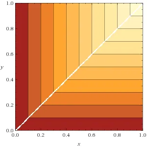
This has too many flat sections and doesn't adequately discrimiate between materials, e.g. \(f(0.1,0.1) = f(0.1,1)\).
Arithmetic average
\(f_{aa}(x,y) = \frac{x + y}{2}\)
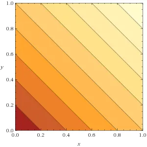
This doesn't favour slippy over grippy enough.
Geometric average
\(f_{ga}(x,y) = \sqrt{{x}{y}}\)
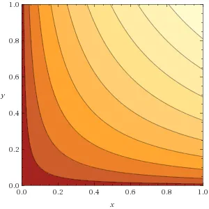
This is good, but the values aren't equally spaced. For this reason, I have found an alternative function - a weighted sum of \(x\) and \(y\).
Weighted sum
\(f_{ws}(x,y) = \frac{{x}{w_{x}} + {y}{w_{y}}}{w_{x} + w_{y}}\) where \(w_{x} = \sqrt{2}(1 - x) + 1\)

\(f_{ws}\) has a more regular spacing between values than \(f_{ga}\). The trade-off is that it doesn't cover the full range of values for \(f(x,1)\) (\(f(0,1) \approx 0.3\)). However, they are approximately equal for \(0.2 \le x \le 1\).
Restitution
As with friction, the minimum, the arithmetic average, and the geometric average are often used.
Minimum

\(r_{min}\) has the same objections as \(f_{min}\).
Geometric average

\(r_{ga}\) is not suitable because it would require the world material to have a restiution near \(1\) to provide a wide range of combined values.
Arithmetic average

\(r_{aa}\) is better, but it doesn't give a very wide range of values for \(r(x,0.5)\). We can improve on this range by allowing some flatness and defining \(r\) as a piecewise min/max/sum function.
Piecewise min/max/sum
\(r_{pmms} = \begin{cases}min(x,y) & \text{if }x \lt 0.5 \land y \lt 0.5\\max(x,y) & \text{if }x \gt 0.5 \land y \gt 0.5\\x + y - 0.5 & \text{otherwise}\end{cases}\)
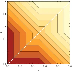
This has the same shortcomings as \(r_{min}\) at the corners where the min and max functions are used. But you can't avoid that if you want to have the full range of values for \(r(x,0.5)\) and still satisfy \(r(x,x) = x\). Similar to the friction, I have created a weighted sum function that I think is better.
Weighted sum
\(r_{ws}(x,y) = \frac{{x}{w_{x}} + {y}{w_{y}}}{w_{x} + w_{y}}\) where \(w_{x} = \sqrt{2}\left\vert{2x - 1}\right\vert + 1\)
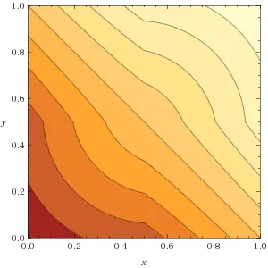
As with \(f_{ws}\), \(r_{ws}\) sacrifices some of the range for \(r(x,0.5)\) to provide better continuity in the corners.
Why \(\sqrt{2}\)?
It's the choice that maximizes the function range, while maintaining monotonicity. These graphs show what \(f_{ws}\) looks like with \(w_{x} = c(1 - x) + 1\), for \(c = 0.5\), \(c = 1\), \(c = \sqrt{2}\), \(c = 2\), and \(c = 4\). For \(c \lt \sqrt{2}\), \(f_{ws}(x,1)\) has less range. For \(c \gt \sqrt{2}\), \(f_{ws}\) is no longer monotonic - near \(f_{ws}(0.1,0.9)\) it starts to curve back, making a more grippy material have a lower combined friction! You can see this more clearly for higher values of \(c\).
\(c = 0.5\)
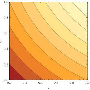
\(c = 1\)

\(c = \sqrt{2}\)

\(c = 2\)
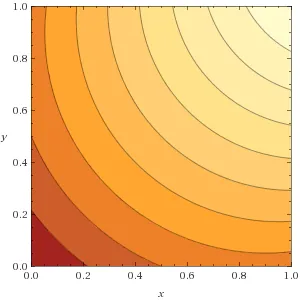
\(c = 4\)
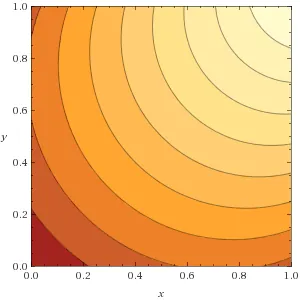
Conclusion
The method to combine material friction and restitution values may seem like a minor detail, but sometimes the devil's in the details.
Since the whole concept of defining values for friction and restitution for a single material and then combining them isn't physically accurate, this is obviously just a case of finding a suitable function rather than attempting to model reality. You may have different requirements for your functions, but I hope this discussion of the alternatives is useful.
Links
I made the graphs at the WolframAlpha web site. I find it's a pretty useful tool. Here's an example plot.


Different physics engines have really different ways of applying those values. It would be interesting to see also some "test case" and few real objects modeled thanks to that model and showing inconsistencies among different physics engines.