This article will explain the theory behind image filtering. Only a few basic filters are discussed; more complex filters will not be dealt with due to their different nature. We will discuss filter design and cover much of the necessary terminology one might come across when reading related literature. Source code is supplied with the article that implements a greyscale edge detection filter.

1: The Terminology

The filter - its properties, characteristics and functionality

First off, what is a filter? A filter is any kind of processing that has one characteristic: it takes a signal as the input and produces a relevant output signal after processing it in some way. A filter can always be mathematically described - think of it as a function, for instance: Fig. 1.1: The least elaborate form of a simple filter that only takes one argument (an input signal or sample) and produces an output signal or sample A filter can take any number of arguments that further define its behaviour - in fact, when designing a filter we usually need to give it a few guidelines according to which it will be built. In this article we will only be dealing with filters that are designed using one parameter - the dimensions - the contents of the filter we will choose carefully ourselves (no mathematical methods are discussed). More on this later. Notice that we defined the dimensions of a filter as one parameter - this hints that most filters have uniform side length. For a 1D filter this will define the length while for 2D filters the dimension will define the length of the sides. In essence one could also create 3D filters, but there aren't that many everyday uses for them. An example of a 1D filter: Fig. 1.2: a 1D filter Notice one very important, although subtle, characteristic in figure 1.2 - the filter has an odd number of samples. This is a must for filters - the sample distribution doesn't have to be symmetrical (although usually it is) across the centre sample, but it must be possible to centre the filter over any sample in an input signal. An example of a 2D filter: Fig. 1.3: a 2D filter A 2D filter, too, has to have an odd number of samples in both the vertical as well as the horizontal orientation. The filters in figures 1.2 and 1.3 are not "real" - they were created randomly.

The spatial, frequency and time domains

The above terms actually define two different "spaces". The catch here lies that while the time domain only exists for 1D signals (such as an audio signal), the spatial domain describes a 2D signal (an image). Both of these domains can be converted into an alternate domain - the frequency domain. The process used to do the conversion is called the Fourier Transform and will not be discussed in this article because it has very little use in image filtering. That is, while most audio filters (high pass, low pass, band pass and others) function in the frequency domain, image information is encoded mostly in the spatial domain, requiring no conversion at all. The moral here - if you look at an image, think of the spatial domain; in the case of an audio signal think of the time domain and when looking at a frequency spectrum (as in WinAMP), think of the frequency domain. For now, let's forget all about everything but the spatial domain.

The kernel and the PSF

Again, these two terms mean the exact same thing with the difference that a kernel generally denotes the use of a 1D filter while the PSF, which stands for point spread function, denotes the use of a 2D filter. There is yet another name that is used: the impulse response, which is arguably the most relevant for both cases. Looking back at figures 1.2 and 1.3, one can see that the explanations below them are flawed. The figures do not show what a filter looks like, but rather the impulse responses of the respective 1D and 2D filters. We will be using all of the terms interchangeably for all filter types.

Convolution as a mathematical operation

Applying a simple filter to an input signal requires some math to be done. The method used for kernel-type filters is called convolution. It is a ternary mathematical operation (taking two arguments and producing one output value) just as addition or multiplication. Compared to the two, however, it is more like multiplication due to one very important characteristic in signal processing: linearity. Linearity There are two types of systems that surround us: a system can either be linear or non-linear. Most real life systems (such as temperature changes) can be characterized as non-linear. This means that there is a lot of uncertainty involved. Mathematics introduces some very well known non-linear operations and functions: integration, division, multiplication, taking the logarithm, etc. This means that it is somewhat challenging to know the source data by analyzing the output data. Fortunately mathematics also introduces inverse functions and operations to most of the commonly used ones: division for multiplication, logarithm for exponentiation, etc. Other types of systems are linear - systems that we can and most of the time do know a great deal about. It isn't uncommon that a linear system is perfectly defined - that is, we know everything about it. Two linear mathematical operations are addition and subtraction. Convolution belongs to the non-linear class - that means that once a signal is convolved, it isn't at all that trivial to reproduce the original signal. Although the inverse of convolution, deconvolution, exists, it is not discussed in this article. In mathematics, convolution is generally denoted with the asterisk (*). This notation is what we will be using so do not confuse it with multiplication! Again, mathematically speaking, here's how the whole thing works: Eq. 1.1: 1D convolution (the black dot denotes multiplication). y is the output signal, x is the input signal and h is the filter kernel Eq. 1.2: 2D convolution Let's explain the above math for two-dimensional signals. First off, we need to view both the input signal and the output signal as well as the filter's impulse response as two dimensional matrices that can be accessed through respective coordinates n and m, i and j. To produce an output sample y[n, m], we multiply a sample and its surrounding samples in the input signal x with corresponding samples in the filter's impulse response h and add the products. Visually, this means that: Fig. 1.4: a convolution example of a 2D signal with a 2D filter with c=-1/8. The asterisk (*), as mentioned above, denotes convolution. By the way, figure 1.4 uses the actual PSF used for edge detection from the code example provided with this article - therefore it is an actually used impulse response. Two very important things can be seen in figure 4. Firstly, convolution with a filter kernel that includes negative values, may produce negative output values. For instance, consider the following: Fig. 1.5: a sample and impulse response combination that produces a negative output value if c < 0 The product of the above convolution for c = -1/8 is , which brings us to the question: what should we do if we encounter negative values? There are two feasible solutions to solve this problem: we could simply discard any values below 0 or we could include a correction factor and shift all of the values in the output signal by some constant - for instance, this could be a constant value added to all of the samples in the output signal. The other important thing to note is the change in data types. Namely, the edge detection used here introduces floating point values which generally also make the output sample a floating point value. The best solution to remedy this is rounding - we simply crop the sample values in the output signal that have a nonzero fractional part. It's as simple as that. Yet another thing worth notice is the fact that convolution is commutative (it doesn't matter if you convolve the input sample with the filter kernel or vice versa - the outcome is the same), associative (if you have three signals, it doesn't matter which two you convolve first) as well as distributive (). Convolving a 1D signal is almost identical to convolving a 2D signal (just lose the extra dimension). We will next look at how to put all of the above together to produce a functioning filter, what problems it will introduce and how to battle them.

2. Filtering an input image

Even though the only limitation for filter dimensions is the fact that it has to have an odd number of samples, problems arise when we use a filter kernel with d > 1 with more than one non-zero value. That is, the only filter that will not introduce artefacts in the output signal is the impulse filter, which has the following kernel: Fig. 2.1: a simple two-dimensional impulse where n?N. If n=1 the impulse response becomes a unity impulse, e.g. it will not change the input signal In the case of a different PSF we will end up with strange artefacts appearing near the edges of the filtered image (the brightness will not be correct). The breadth of these un-normalized regions will depend on the size of the filter kernel. Although neither the sample code nor the sample application provided with this article address this issue, the solution to this problem is relatively simple: for all output image samples that lie near the edge of the image so that parts of the filter kernel are clipped outside of the image boundaries, count the number of impulse response samples that are clipped and divide the output sample by the fractional part of the non-clipped samples compared to the used samples. That is, if in a 3x3 PSF only 4 samples are used to calculate the output sample value, divide the latter by the overlapping fraction of 4/9. Some filters produce an output that may require special handling after filtering. For instance, the emboss filter will surely produce a lot of negative values which means that it would be wise to add some constant to the output samples. After some experimenting, you might find that 128 seems like a nice number. In the code sample provided with this article (implementing the edge detection filter) we're multiplying the resultant sample by 9. Why nine? The answer is: pure experimentation! This solves the problem with clipping negative numbers, but yet another (although somewhat insignificant) problem remains. Since, we're dealing with floating point numbers, our sample values aren't always nicely spaced out between 0 and 256. Instead, some of them may be larger than 255. For this we've introduced a ceiling boundary - anything above 255 is simply discarded. Equipped with this knowledge, we're now almost ready to produce a working filtering program. Still, there remains the question of how do we come up with the appropriate filter design?

3. Designing a filter

This may seem surprising, but high-profile filter design comprises 40% logic and predicate analysis and 60% experimentation. We will now look at different filters commonly used and the changes they introduce if we vary some parameters. To demonstrate a possible output of the following filters we will be applying them to this source image: Img 3.1: the original reference image used hence forth

Since the sample program accompanying this article only handles greyscale images (that are converted into 24 bit DIB's upon export), the reference images produced in Paint Shop Pro 4.12 have first been converted to greyscale and then filtered.

Even though the images produced by Paint Shop Pro are interchangeably similar to the ones produced by our software, notice the discrepancies at the edges of the images we've presented - this "artefact" has been discussed above. Just know that it is not a bug!

Edge detection

The single most important feature one could extract from an image is the edge data. The edge information can be parallelized to the frequency spectrum of an audio signal - one can use it to do a lot of very neat tricks with the image. For instance, if the edges are fuzzy and hard to make out, a modified version of edge detection - edge enhancement - can be used to enforce the contours. Edge detection is the most important thing in image recognition - for instance, if we have a reference image and some target image that we want to locate (or verify if it exists) in the reference image, we first find the edges in both images and do a check using the edge data instead of some weird interpolation that uses pixel information. Cell shading can be accomplished through edge detection - a neat effect to be used in games. Once again, the kernel of a traditional edge detection filter looks like this (this has been covered above): Fig. 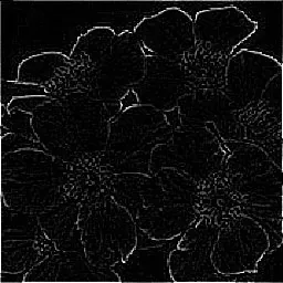3.1: the traditional filter kernel of an edge detection filter where c = -1/8 Here are the output images: [nbsp][nbsp] 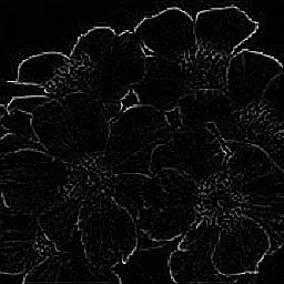Img 3.2: comparing our output image (left) to the one produce by Paint Shop Pro (first made greyscale, then applied with Image->Edge Filters->Find Edges). Paint Shop Pro also has Find Horizontal/Vertical Edges which will be left up to you to design

Edge enhancement

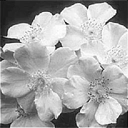
If we're only stuck with a blurry image, we can use a parameterized edge detection filter to make the edges stick out more. To do this, we modify the constant c in the edge detection filter with the value c = -k/8. Here are the results: [nbsp][nbsp] 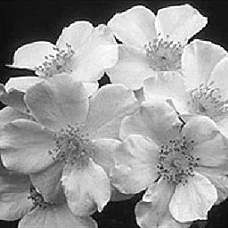Img 3.3: the edge enhancement filter does nothing more than makes the edges in the image more prevalent. We used k = 3 in this case

Sharpen and unsharpen (blur)

Sharpening is pretty much the same as edge enhancement - it accentuates the edges, unsharpening, or blurring, being its immediate inverse. We won't be comparing the output images for these filters as we're not using the same constants as Paint Shop Pro (our filter sharpens more at a time). Here are the filter kernels used: Fig 3.1: the sharpening filter kernel. We're using c=-1 in the sample software Fig 3.2: the unsharpening filter kernel

Emboss and engrave

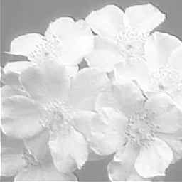
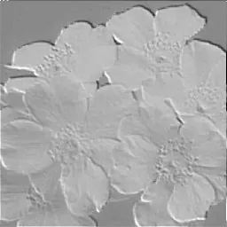
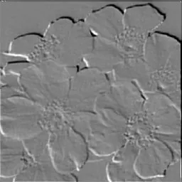
Embossing is probably one of the 'coolest' effects that can be applied to an image. Its close relative, bumpmapping, is one of those few texture effects that you can often toggle on and off in a game. Bumpmapping relies on the presence of a "bump image", or the bump map which is essentially nothing more than a simple embossed image that can be created using your favourite image editing program. By combining this bump image with the texture map you can create the final bumpmapped image. Using what we've learnt so far, it isn't difficult to construct a simple embossing filter that does the whole business of creating the bump image for us without the need for fancy software. Here is a set of the filter kernels used for embossing an image: Fig 3.3: a 3x3 emboss filter kernel Fig 3.4: a 5x5 emboss filter kernel Fig 3.5: a 7x7 emboss filter kernel The following image listing shows how these filters perform and how we should go about trying to create some very specific effect. [nbsp][nbsp] [nbsp][nbsp] 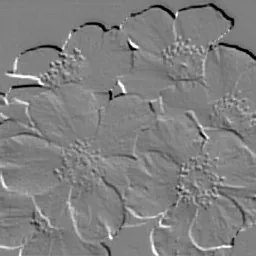Img 3.4: using different filter kernel sizes creates different depths in the embossed image. Can you hazard a guess which kernel size Paint Shop Pro might be using? (images counter-clockwise from top right: 5x5 filter kernel, 3x3 filter, 7x7 filter and PSP) "Fine," you say, but what's up with the above images - why is the intrinsic brightness of the images so different? The reason is simple - we're using a constant correction factor of 128 (as reasoned in section 2) for all three filter sizes (after filtering each pixel, we add 128 to its value to compensate for the negative output sample values). The fewer negative numbers there are in the filter the more positive the output sample values will be, meaning that smaller filters produce inherently brighter images and should therefore have a smaller correction value. It will be left up to you to figure out how to obtain the correction values dynamically. Now from emboss to engrave - these two seem like opposites while, in fact, we can solve the problem with a simple visual "hoax". Try turning any of the embossed images upside down and have a look at it. Most people now see the image as "dented" - having depression areas rather than a hilly look. This can be thought of as changing the direction of the incident light - if we were to rotate the negative values around the central 1, we'd be seeing the image differently - at one point it would simply go from "embossed" to "engraved". There are other filters that can be implemented using this simple method (convolution), but they won't be discussed in this article. More complex filters, such as artistic filters, cannot be implemented that easily and often require huge amounts of research and experimentation to get to work right. With the filters described above, however, one could do a whole world of things. There are a few points to keep in mind, though - these will be discussed in the next section.

4: Do's and don'ts and a few clarifications

Speed issues

At current time, implementing real-time filtering is pretty much out of the question. Once the kernel size is pushed upwards of a few samples, speed issues really start to kick in. For instance, convolving a 1024x1024 image with a 64x64 filter kernel, 1024x1024x64x64 (it is a 10-digit number) floating point multiplications and additions would have to be done. There is a way to slacken this situation using FFT (Fast Fourier Transform) convolution, but it won't be discussed here. There are a few but's for FFT convolution as well, anyway... The moral is to always be wary when an image has to be filtered - even on today's high-end systems a large image could take more than several seconds to process using a small filter kernel.

It's all about experimentation

The discussed filter kernels (those introduced in section 3) resulted largely from experimentation and were implemented as static filters (that means no mathematical algorithm was developed to compute them in any size). Coming up with such algorithms can sometimes be rather challenging.

The hidden equilibrium

It isn't that obvious, but a certain kind of "numeric balance" hides itself in filters. If the balance is shifted, the filter starts to distort the image instead of simply processing it. That is, if adding all of the values in a filter kernel together produces a value that doesn't equal 1, the filter is "numerically unbalanced". For instance, figure 3.1 presents a neatly balanced filter while the kernel presented in 3.5 is an unbalanced one. This knowledge serves no practical purpose, but it can be used to assess the "rate of distortion" of a filter.

What is the 'normal' filter size?

This is a fair question that can be answered in the following way: for most applications the very primitive 3x3 filter kernel is more than enough; larger filters become necessary when the output sample needs to be affected by a whole area of surrounding pixels. For instance, increasing the kernel size of the emboss/engrave filter produces an increasingly embossy/engravy effect. Implementing a large median filter (used for removing small artefacts such as speckles from the input image - not done by convolution) will yield an increasingly blurrier while smoother output image.

5: Conclusion

The use of filters in everyday life is pretty concealed. Nevertheless, we couldn't exist if it weren't for filters - they are a product of nature (our eyes and ears silently use them for audio and visual object recognition, for feature enhancement - such as identifying objects in low-level light and a ton of other purposes that most people aren't even aware of) that have been successfully incorporated into technology (one can find numerous filters in the computer next to him or herself, in any electronic music instrument, etc). Image and other filtering techniques can be abusively complex - the mathematical theory behind them spans much further than the simple operation of convolution. This article has been a taste of the easy cream coating on top of hardcore DSP techniques used for optimally fast and effective image manipulation.

Addendum: The accompanying software and source code example

All of the filters discussed here and a few others are implemented in the sample application supplied with this article. There are a few things to keep in mind when filtering images with it or the simple code sample provided. They can only be uncompressed 24 bit bitmaps (either greyscale or color); the output images will always be 24 bit bitmaps converted to greyscale (all color components of a pixel are give the same value). The source code sample is fully documented and implemented as a command line application - see the accompanying edge_detect.txt for instructions on how to use it. The source code was written in Borland C++ 5.02 and will most likely not compile on non-Borland compilers - a few minor adjustments need to be made on your behalf. Very simple modifications should be enough to make the source sample apply a different filter to the input image. I hope you've found this article to be of some use - if you noticed a mistake or have any questions/comments you'd like to share, contact me at [email="christopheratkinson@hotmail.co.uk"]christopheratkinson@hotmail.co.uk[/email].