Abstract Using a neural network for the brain, we want a vehicle to drive by itself avoiding obstacles. We accomplish this by choosing the appropriate inputs/outputs and by carefully training the neural net. We feed the network with distances of the closest obstacles around the vehicle to imitate what a human driver would see. The output is the acceleration and steering of the vehicle. We also need to train the network with a set of strategic input-output. The result is impressive, for a couple of neurons! The vehicle drives around avoiding obstacles, but some improvement or modification can be done to make this software work for a specific purpose. Introduction The idea is to have a vehicle that drives by itself and avoids obstacles in a virtual world. Every instant, the vehicle decides by itself how to modify its speed and direction according to its environment. In order to make it more real, the AI should only see what a person would see if it was driving, so the AI's decision is only based on obstacles that are in front of the vehicle. By having a realistic input, the AI could possibly be used in a real vehicle and work just as well. Gaming is the first use I think of when I hear "AI controlling a vehicle". Many driving games could use this technique to control vehicles, but there are a number of other applications that could be found for software that controls a vehicle in a virtual world, or in the real world. So how do we do this? There are many AI techniques out there, but since we need a "brain" to control the vehicle, neural networks would do the job. Neural networks are based on how our brain works; they seems to be the right choice. We will need to define what the input and output should be for this neural network. Neural Networks The Neural Network Artificial Intelligence comes from how brains work. Our brain is composed of 10[sup]11[/sup] neuron cells that send electrical signal to each other. Each neuron is composed of one or two axon which work as output and many dendrites which work as input of electrical signals. Neurons need a certain strength of signal input that adds up from all the dendrites to be triggered. Once triggered, the neuron will fire and send an electrical signal down its axon to other neurons. Connections (axon and dendrites) will strengthen if they are often used. This principle is applied to neural networks on a smaller scale. Today's computers don't have the power of computing that 20 billion neurons do, but even with a few neurons, we are able to have intelligent response from a neural network. Neurons are organized in layers as figure 1 shows. The input layer will have entries, and depending on the strength of connection to each neuron in the next layer, the input signal is sent to the next layer. The strength of the connection is called a weight. The value of each neuron in each layer will depend on the weight of the connection and the values of the neurons of the previous layer.
Neural Networks The Neural Network Artificial Intelligence comes from how brains work. Our brain is composed of 10[sup]11[/sup] neuron cells that send electrical signal to each other. Each neuron is composed of one or two axon which work as output and many dendrites which work as input of electrical signals. Neurons need a certain strength of signal input that adds up from all the dendrites to be triggered. Once triggered, the neuron will fire and send an electrical signal down its axon to other neurons. Connections (axon and dendrites) will strengthen if they are often used. This principle is applied to neural networks on a smaller scale. Today's computers don't have the power of computing that 20 billion neurons do, but even with a few neurons, we are able to have intelligent response from a neural network. Neurons are organized in layers as figure 1 shows. The input layer will have entries, and depending on the strength of connection to each neuron in the next layer, the input signal is sent to the next layer. The strength of the connection is called a weight. The value of each neuron in each layer will depend on the weight of the connection and the values of the neurons of the previous layer.
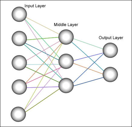 Figure 1: Basic Neural Network
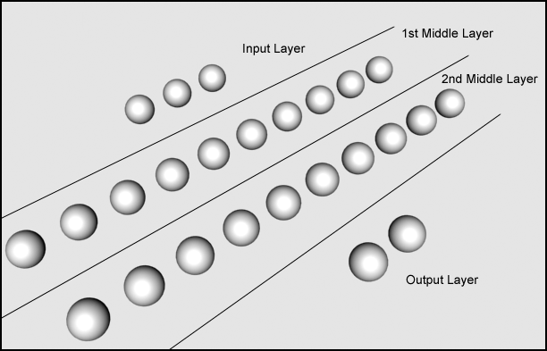 Figure 2: 3-8-8-2 Neural Network
The Input What information is important in controlling a vehicle when we are driving? Firstly, we need the position of obstacles relative to us. Is it to our right, to our left or straight ahead? If there are buildings on both side of the road, but none if front, we will accelerate. But if a car is stopped in front of us, we will brake. Secondly, we need the distance from our position to the object. If an object is far away we will continue driving until it is close, in which case, we will slowdown or stop. That is exactly the information that we use for our neural network. To keep it simple we have three relative directions: left, front and right. And we need the distance from the obstacle to the vehicle.
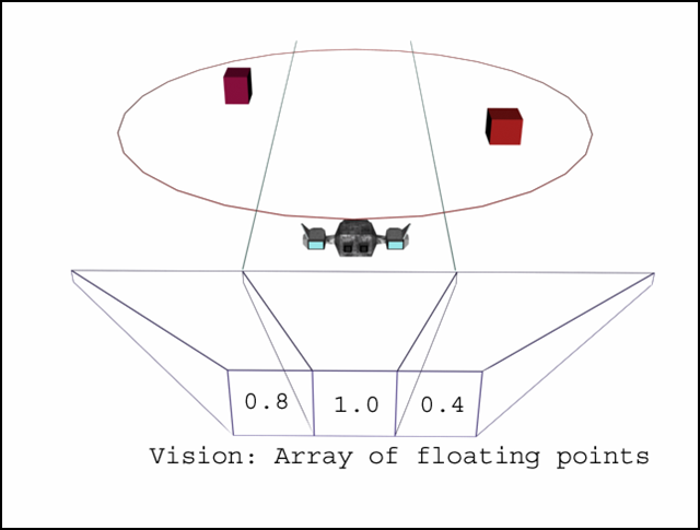
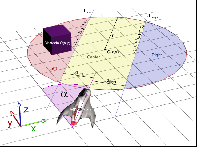
We will define what kind of field of vision our AI driver should see and make a list of all the objects it can see. For simplicity we are using a circle in our example but we could use a real frustum with 6 intersecting planes. Now for each object in this circle, we check to see if it is in the left field of view, right field of view or center. The input to the neural network will be an array: float Vision [3]. The distance to the closest obstacle to the left, center, and right of the vehicle will be stored in Vision [0], Vision [1] and Vision [2] respectively. In Figure 3, we show how the array works. The obstacle on the left is at 80% of the maximum distance, the obstacle on the right is at 40% of the maximum distance and there is no obstacle in the center. To be able to do this, we need the position (x,y) of every object, the position (x,y) of the vehicle and the angle of the vehicle. We also need 'r' (the radius of the circle) and d[sub]right[/sub], d[sub]left[/sub], the vectors from the craft to the lines L[sub]right[/sub], L[sub]left[/sub]. Those lines are parallel to the direction of the craft. Both vectors are perpendicular to the lines. Even though it is a 3D world, all the mathematics is 2D because the vehicle doesn't go into the 3[sup]rd[/sup] dimension since it is not flying. All the equations will only consider x and y and not z. First, we compute the equations of the lines L[sub]right[/sub] and L[sub]left[/sub] which will help us determine whether an obstacle is to the left, right or center of the vehicle. Check figure 4 for an illustration of all the variables. with
with  Then we compute a point on the line
  with V[sub]x[/sub], V[sub]y[/sub] the position of the vehicle. Then we can finally compute c[sub]R[/sub]
  We proceed the same way to compute the equation of the line L[sub]left[/sub] using the vector d[sub]left[/sub]. Second, we need to compute the center of the circle. Anything within the circle will be seen by the AI. The center of the circle C(x,y) is at the distance r from the vehicle's position V(x,y).
 with V[sub]x[/sub], V[sub]y[/sub] the position of the vehicle and C[sub]x[/sub], C[sub]y[/sub] the center of the circle. Then we check every object in the world to find out if they are within the circle (if the objects are organized in quadtree or octtree, the process is much faster than with a linked list). If
  then the object is within the circle, with O[sub]x[/sub], O[sub]y[/sub] the position of the obstacle. For every object within the circle, we then must check if they are to the right, left or center of the vehicle. If
  then the object is in the right part of the circle else if
  then the object is in the left part of the circle else it is in the center. We compute the distance from the object to the vehicle
  Now we store the distance in the appropriate part of the array (Vision[0], Vision[1] or Vision[2]) only if the distance already stored is larger than the distance we just computed. The Vision must have been initialized to 2r prior to that. After checking every object, we have the Vision array with the distance to the closest object to the right, center and left of the vehicle. If no object were found for one of those sections, we will have the default value
  which means: "no object in view". Because the neural network is a using a sigmoid function, the input needs to be between 0.0 and 1.0. 0.0 should mean that an object is touching the vehicle and 1.0 means that there is no object as far at it can see. Since we set a number for the maximum distance the AI driver should see, we can easily modify all the distances to a floating point between 0.0 and 1.0.
The output The output needs to control the vehicle's speed and direction. That would be the acceleration, the brake and the steering wheel. So we need 2 outputs; one will be the acceleration/brake since the brake is just a negative acceleration, and the other will be the change in direction. The output from the neural network is also between 0.0 and 1.0 for the same reason as the input. For the acceleration, 0.0 means "full brakes on"; 1.0 means "full gas" and 0.5 means no gas or acceleration. For the steering, 0.0 means full left, 1.0 means full right and 0.5 means strait ahead. So we need to translate the output into values that can be used. 
 We should note that a "negative acceleration" means braking if the vehicles is moving forward, but it also means going into reverse if the vehicle is at rest. Similarly, a "positive acceleration" means braking if the vehicle is moving in reverse.
 Training As I mentioned earlier, we need to train the neural network to approximate the function we need it to accomplish. We need to create a set of input-output that would be the main reaction we want the neural network to have. Choosing the right input-output to train a neural network is probably the trickiest part of all. I had to train the network with a set of input-output, see how it reacted in an environment, and modify the entries as needed. Depending on how we train the network, the vehicle can hesitate in some situations and get immobilized. We make a table (Table 1) with different arrangements of obstacle positions relative to the vehicle and the desired reaction from the AI. Table 1
| Input Neurons Relative distance to obstacle | Output Neurons | |||
| Left | Center | Right | Acceleration | Turn |
| No obstacle | No obstacle | No obstacle | Full Acceleration | straight |
| Half way | No obstacle | No obstacle | Accelerate a bit | Little bit to the right |
| No obstacle | No obstacle | Half way | Accelerate a bit | Little bit to the left |
| No obstacle | Half way | No obstacle | Slow down | Little bit to the left |
| Half way | No obstacle | Half way | Accelerate | straight |
| Touching Object | Touching Object | Touching Object | Reverse | Left |
| Half way | Half way | Half way | No Action | Little bit to the left |
| Touching Object | No obstacle | No obstacle | Slow down | Full Right |
| No obstacle | No obstacle | Touching Object | Slow down | Full Left |
| No obstacle | Touching Object | No obstacle | Reverse | Left |
| Touching Object | No obstacle | Touching Object | Full Acceleration | straight |
| Touching Object | Touching Object | No obstacle | Reverse | Full Right |
| No obstacle | Touching Object | Touching Object | Reverse | Full Left |
| Object Close | Object Close | Object Very Close | No Action | Left |
| Object Very Close | Object Close | Object Close | No Action | Right |
| Touching Object | Object Very Close | Object Very Close | Slow down | Full Right |
| Object Very Close | Object Very Close | Touching Object | Slow down | Full Left |
| Touching Object | Object Close | Object Far | No Action | Right |
| Object Far | Object Close | Touching Object | No Action | Left |
| Object Very Close | Object Close | Object Closer than halfway | No Action | Full Right |
| Object Closer than halfway | Object Close | Object Very Close | Slow down | Full Left |
| Input Neurons | Output Neurons | |||
| Left | Center | Right | Acceleration | Turn |
| 1.0 | 1.0 | 1.0 | 1.0 | 0.5 |
| 0.5 | 1.0 | 1.0 | 0.6 | 0.7 |
| 1.0 | 1.0 | 0.5 | 0.6 | 0.3 |
| 1.0 | 0.5 | 1.0 | 0.3 | 0.4 |
| 0.5 | 1.0 | 0.5 | 0.7 | 0.5 |
| 0.0 | 0.0 | 0.0 | 0.2 | 0.2 |
| 0.5 | 0.5 | 0.5 | 0.5 | 0.4 |
| 0.0 | 1.0 | 1.0 | 0.4 | 0.9 |
| 1.0 | 1.0 | 0.0 | 0.4 | 0.1 |
| 1.0 | 0.0 | 1.0 | 0.2 | 0.2 |
| 0.0 | 1.0 | 0.0 | 1.0 | 0.5 |
| 0.0 | 0.0 | 1.0 | 0.3 | 0.8 |
| 1.0 | 0.0 | 0.0 | 0.3 | 0.2 |
| 0.3 | 0.4 | 0.1 | 0.5 | 0.3 |
| 0.1 | 0.4 | 0.3 | 0.5 | 0.7 |
| 0.0 | 0.1 | 0.2 | 0.3 | 0.9 |
| 0.2 | 0.1 | 0.0 | 0.3 | 0.1 |
| 0.0 | 0.3 | 0.6 | 0.5 | 0.8 |
| 0.6 | 0.3 | 0.0 | 0.5 | 0.2 |
| 0.2 | 0.3 | 0.4 | 0.5 | 0.9 |
| 0.4 | 0.3 | 0.2 | 0.4 | 0.1 |
Conclusion / Improvement Using a neural network with back propagation works well for our purposes, but there are some problems once implemented and tested. Some improvement or modification can be done to either make the program more reliable or to adapt it to other situations. I will now address some of the problems you might be thinking about right now.
Figure 5
The vehicle does get "stuck" once in a while because it hesitates deciding whether it should go right or left. That should be expected: humans have the same problem sometimes. Fixing this problem is not so easy if we try to tweak the weights of the neural network. But we can easily add a line of code that says: "If (vehicle doesn't move for 5 seconds) then (take over the controls and make it turn 90 degrees right)". With this simple check, we ensure that the vehicle will never get in a place not knowing what to do. The vehicle will not see a small gap between two buildings as shown in figure 5. Since we don't have a high level of precision in the vision (left, center, right), two buildings close together will seems like a wall for the AI. To have better vision of our AI, we need to have 5 or 7 levels of precision in the input for the neural network. Instead of having "right, center, left" we could have "far right, close right, center, close left, far left". With a careful training of the neural network, the AI will see the gap and realize that it can go through it. This works in a "2D" world, but what if we have a vehicle capable of flying through a cave? With some modification of this technique, we can have the AI fly rather than drive. Similar to the last problem, we add precision to the vision. But instead of adding a "far right" and a "far left", we can do as shown in Table 3. Table 3 [table][tr] [td]Upper left[/td] [td]Up[/td] [td]Upper right[/td] [/tr] [tr] [td]Left[/td] [td]Center [/td] [td]Right[/td] [/tr] [tr] [td]Lower left[/td] [td]Down[/td] [td]Lower right[/td] [/tr] [/table] All the vehicle does is "wander around" without purpose. It doesn't do anything other than avoiding obstacle. Depending on why we need an AI driven vehicle, we can "swap" brains as needed. We can have a set of different neural networks and use the right one according to the situation. For example, we might want the vehicle to follow a second vehicle if it is in its field of view. We just need to plug another neural network trained to follow another vehicle with the position of the second vehicle as input. As we have just seen, this technique can be improved and used in many different areas. Even if it is not applied to any useful purpose, it is still interesting to see how an artificial intelligent system reacts. If we watch it long enough, we realize that in a complex environment, the vehicle will not always take the same path and because of the small difference in decision due to the nature of neural network, the vehicle will sometimes drive to the left of a building, and sometimes to the right of the same building.